Labs is the research arm of Thinkst but research has always been a key part of our company culture. All Thinksters are encouraged to work with Labs on longer term projects. These become that Thinkster’s “day job” for a while. (These are intended both for individual growth, and to stretch ourselves into new areas: They don’t have to be related to Canary or security).
I took a brief hiatus from the engineering team to explore a computer vision project: CourtVision.
CourtVision set out to explore how to process a video stream of a racquet and ball game (padel–popular in the southern hemisphere and growing in popularity world-wide!) from a stationary (but unaligned) camera and extract information about the game. Padel, like other racquet sports, is played on a regulation court with lines demarking in and out of bounds (though there are times when a ball is in play even outside of the court); CourtVision aimed to extract information such as player positions and ball trajectories from a video feed. Secondly, visualising these outputs to provide insights into game tactics and strategies.
While there are existing computer vision systems to track play in racquet games, namely the Hawk-Eye system, these require systems of multiple fixed, calibrated, and synchronised cameras. The CourtVision challenge was to offer similar outputs from a single viewpoint, that is not in a specific location in relation to the court
The problem formulation
The problem is thought of as unwinding the events that gave rise to the video. To achieve this we draw on prior knowledge such as court layout and ball and player dynamics. At each moment during a game the light emanating from the scene is sampled (at 30 fps) and produces a sequence of images.
The problem now is to associate certain pixels in the image with objects in the scene we would like to know more about and then make estimates about the objects positions that best explain the sensor readings – image sequence.
Starting from here a number of avenues were explored and below is a linearized path of how we went about solving this problem.
The path is simple (looking back):
- Establish a mapping from world coordinates to image plane pixel locations.
- Detect objects of interest (players and ball) in each frame.
- Estimate the world coordinates of each object by leveraging the inverse mapping found in Part 1.
Establishing a mapping between world coordinates and image plane is a well understood problem and implementations exist in commonly used computer vision libraries. The unknown in our case is doing it given a single image. Taking inspiration from [3], where they used the net on a tennis court to form an additional plane, we took orthogonal planes from the court structure and jointly found the camera pose and intrinsic matrices. This is explained in Part 1of the blog below.
In Part 2 we expand on how we leveraged existing computer vision models to detect objects of interest in each frame.
Previous works that attempted 3D tracking from a single camera relied on either: knowing the size of the object being tracked [1] and that its projected size is invariant to the viewing angle i.e spherical objects; or the object of interest followed purely ballistic trajectories [2]. Here, we modeled the ball trajectory as a ballistic trajectory but retained a multimodal distribution over the ball’s states in a particle filter allowing the tracker to quickly adapt to new trajectories (modes) without explicitly modeling the interaction with walls, floor and racket. Part 3 illustrates this approach.
We made the following assumptions:
- Camera is stationary (but does not need to be in a specific location)
- Court dimensions are known.
Players’ feet remain on the ground. Part 3 illustrates limitations in our tracker and by making this assumption we could improve player tracking stability.

Part 1: Camera calibration and pose estimation
Extracting real-world measurements from a camera requires knowing both the extrinsics (position and pose) and the intrinsics (such as focal length and distortion coefficients) of the camera. Once these are known we can map any point in the world coordinate frame to a pixel location in the image. We can also project rays into the world coordinate system from a desired pixel location.
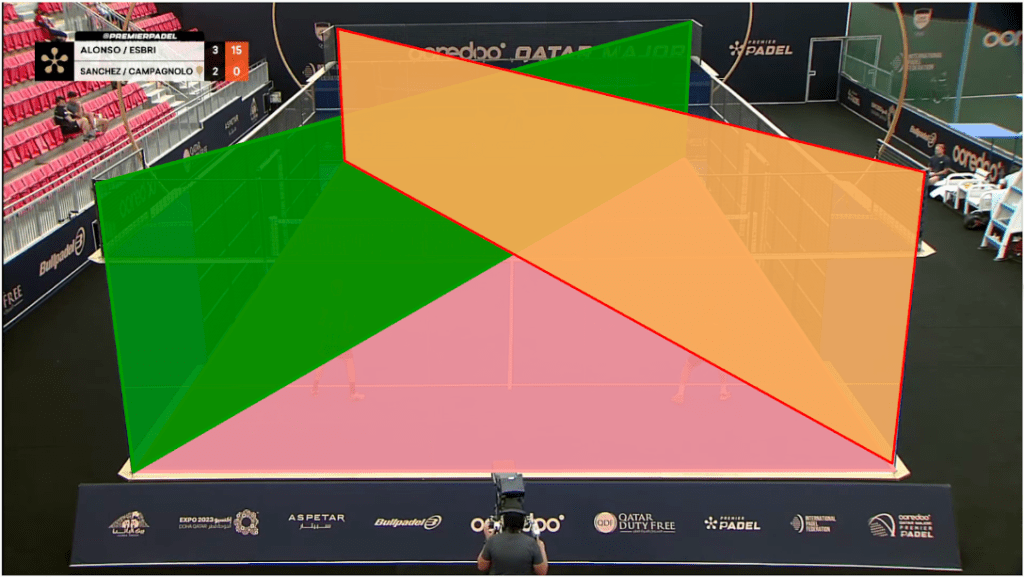
The trade off made for not having to collect data first hand is that little is known about the setup. In this case the camera intrinsics and extrinsics were unknown. The common approach to determine camera intrinsics is to capture a calibration sequence which is often a checkerboard pattern. Since we didn’t have such a luxury we exploited the structure in the scene and defined a set of planes for which the image plane and world coordinate correspondences could be identified. By doing this we effectively introduced a set of 8 planes (similar to a checkerboard) and performed camera calibrations from this. The mean reprojection error was approximately 9 pixels on 1080 x 1920 images.
Part 2: Bootstrapping custom object detectors
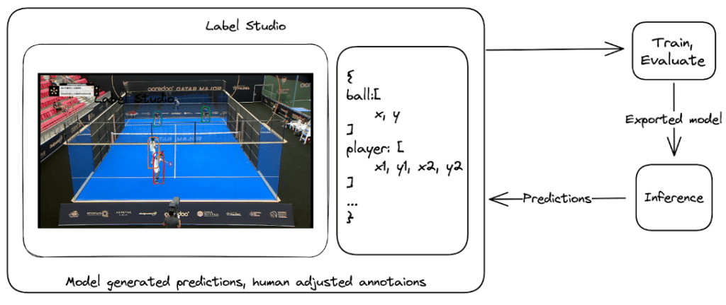
There are a plethora of off-the-shelf models that can do object detection however, none have single class “padel ball” detectors. Fine-tuning such a model is fairly common and to achieve this a few annotated frames were needed. LabelStudio is a very versatile data labeling tool that makes it easy to “put a model in the loop”. By doing this we bootstrapped our ball detector by repeatedly annotating more images and each time using the latest model to automatically label the additional images that were manually verified and corrected.
Part 3: Bringing image detections to the real world
Making detections on an image plane tells us nothing about the player and balls position in the real world. To estimate the position of the ball and players we define a state for each player and the ball and then update this state based on the detections. To govern this process in a more principled manner we used a Bayesian filter and in particular a particle filter.
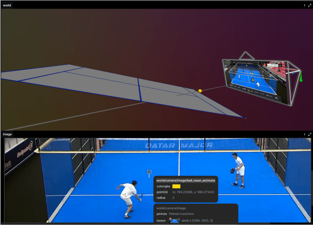
A particle filter stores a distribution over the state of each object. This is stored as a vector and an associated weight indicating a probability mass. To illustrate this the top image in figure 4 shows the cloud of particles representing the state of the ball. During the filter’s update step we follow Bayes rule to update the weight of each particle based on how well they explain the observation (the image). As we can see the core of the particle cloud is around the ray emanating from the detected ball position in the image. All particles along that ray “explain” the observation equally well. The information held in that current state (prior) ensures the updated state does not naively squash all particles onto the ray. Bayesian filters like this are a great way to encode knowledge we have about the ball dynamics and current state and update this belief as we get more observations.

But we don’t want a fuzzy cloud around where the tracker “thinks” the ball is? We want to know the best estimate of the ball’s position. Once again we consult our probability distribution over our ball states. We can grab any statistic we want. The particle with the largest weight – argmax or the weighted mean over all states. Below is the weighted mean position of the ball.
This approach shows promising results but we did see the tracker fail after a few missed detection and resulted in mode collapse. That is the distribution over ball state (cloud of particles as in figure 6) either dispersed or reduced to a point. Particle filters come in a number of flavors and we only implemented the simplest resampling methods so it might be a bug in this or just a naive choice somewhere. Ah, research, so many avenues to explore!
To constrain the player tracking to a plane we called on assumption 3. from above and projected the ray to intersect with the ground plane. These results are shown below as a heatmap of player positions and velocity. Tracking under this constraint means a detected player (measurement) can be projected onto the ground plane (tracker state) with no information loss (3D to 2D) and our tracker remains performant.
Results
The ultimate goal of such a system is to provide insights into game play and strategies. To this end we show court occupation and player movement speeds. The position and velocity heatmaps of players during a rally. The bottom image has Team A in the foreground and Team B in the background. Here we can see where players were during the rally as well as how they moved. In this rally we can see Team A (on the left) plays from deep while Team B (on the right) occupies the mid court far more. Translating this raw positional information into actionable insights remains as future work.
Going from a set of hypotheses to evaluating them is a fun technical challenge and my time in Thinkst Labs was great. I still hope to bring this to a court sometime soon and test the final assumption: seeing game play metrics can improve tactics.
Resources
A collection of tools this project found useful as well as outputs from this work.
- Great computer vision libraries:
- An amazing visualization tool ReRun
- Slick tool for writing type set documents Typst
- Paper (pre-print) describing this work in detail
- Code associated with this project – CourtVision
References
[1] 3D Ball Localization From A Single Calibrated Image
[2] MonoTrack: Shuttle trajectory reconstruction from monocular badminton video
[3] Generic 3-D Modeling for Content Analysis of Court-Net Sports